1-2. Differences between Conventional Calculation (ABC Analysis) and Tera Calculation
In modern logistics facility planning, it is impossible to optimally design increasingly sophisticated distribution centers merely by aggregating past data. In Tera calculation, the conventional rank-based aggregation method utilizing ABC analysis, which has been used on-site for many years, is referred to as "conventional calculation".
This section clarifies the limitations of conventional ABC analysis, which causes the fragmentation of data meaning, and deeply explains the differences in Tera calculation's unique "EIQ Matrix Aggregation" developed to overcome these limitations, as well as the data analysis concepts needed to derive more accurate facility scale calculations.
1. Differences in Basic Concepts between Conventional Calculation and Tera Calculation
Limitations of Conventional Calculation (ABC Analysis) and Information Fragmentation
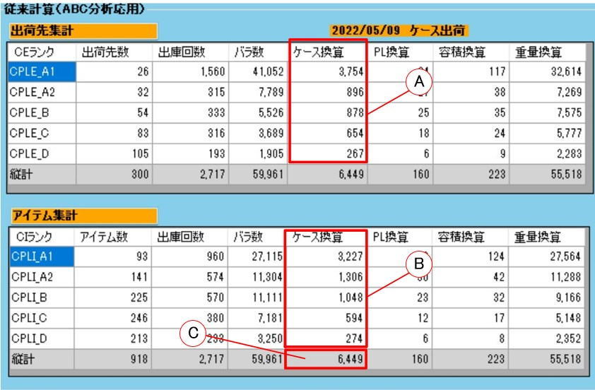
Conventional ABC analysis is a method that independently aggregates item data (best-sellers vs. slow-movers) and shipping destination data (large-lot vs. small-lot) into 3 ranks of A, B, and C based on shipping records. This method is suitable for observing the "distribution of results" for each, and the grand total values of the two tables match.
However, its biggest flaw is that there is absolutely no correlation between the tables. As a result, it is impossible to grasp the three-dimensional structure of "to what proportion are the ultra-best-selling products of item rank A allocated to which shipping destination rank (e.g., large wholesalers or small individual customers)." When this information is missing, it is impossible to accurately measure the appropriate area of the picking zone or the introduction effect of automated equipment like sorters, rendering it insufficient as foundational data for optimal logistics facility planning and operational reviews.
Tera Calculation's Proposal: The "EIQ Matrix Table" for Correlating Data
To resolve this "information fragmentation," Tera calculation expands the ranks into a more precise 5 divisions (A1, A2, B, C, D), and adopts a method of cross-tabulating and correlating by dividing the data into a grid of 25 blocks representing Item Rank (5) × Shipping Rank (5). This is called the "EIQ Matrix Table".
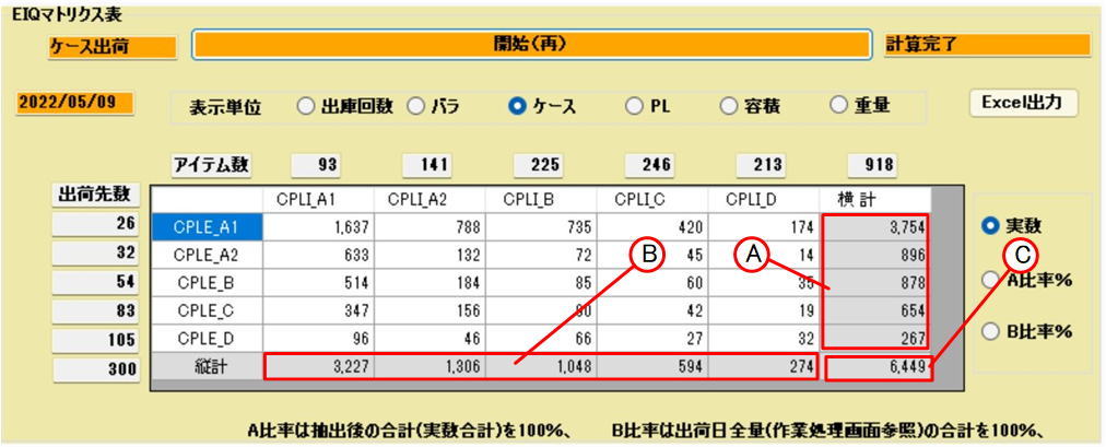
Its greatest feature is the ability to freely switch and display indicators essential in the logistics field—such as "number of lines (retrieval count)," "piece count," "case equivalent," "PL (pallet) equivalent," "volume equivalent," and "weight equivalent"—within the same rank boundaries. This enables a three-dimensional visualization of the required volume for each work area (e.g., how many times picking occurs in which zone, how many cases are needed for replenishment, how many pallets are required for transport), making highly accurate simulations possible.
2. The Importance of the EIQ Matrix Aggregation Table and Visualization
Item 1: The Role of the EIQ Matrix Aggregation Table and Enhanced Readability
- Ensuring consistency with display unit conversion rules:
In the EIQ matrix, the display units of case, PL, volume, and weight are all converted values calculated from the base "piece count." Consequently, the horizontal total of the matrix table always links to the "item aggregation" of the conventional calculation, and the vertical total links to the "shipping destination aggregation," perfectly guaranteeing the matching (consistency) of the entire data.
- Intuitive understanding through grouping massive data:
The original raw EIQ table (e.g., 400 shipping destinations × 4000 items) is so massive that it cannot be fully scrolled through even in spreadsheet software, and the human eye cannot discern trends, causing readability to drop significantly. Tera calculation groups this into 5×5 ranks (EIQ matrix table) to enhance practicality, allowing management and on-site workers to grasp the situation at a glance. Additionally, it can be output as an "EIQ Scatter Plot" that visually confirms the spread of distribution on the screen, supporting intuitive analysis.
Item 2: The Importance of "Tera Setting" in Facility Scale Calculation
When selecting logistics equipment (for example, determining the hourly processing capacity of a sorter), it is common to refer to the peak volume to prevent bottlenecks. However, our institute's ironclad rule is that when calculating the facility scale of a distribution center, which determines the building area and the total number of storage racks, the "overall average of shipping data (Tera Setting)" that is not biased toward specific days should be adopted.
- Reason 1 to avoid specific peak days (Comprehensiveness of all items): If the calculation only extracts specific shipping days, information on items that coincidentally had no shipments on that day (e.g., long-tail products) will be omitted, which severely distorts the evaluation of liquidity and storage efficiency for the warehouse as a whole. By targeting all data (Tera setting), the movements of all items can be accurately comprehensively covered.
- Reason 2 to avoid specific peak days (Prevention of overinvestment): As a basic principle of logistics, the abnormal volume increase during peak shipping times should generally be absorbed temporarily through operations such as advance shipping from safety stock or utilizing additional personnel. If logistics facility planning is based on this peak, the building area and fixed facilities of the center itself will become oversized (over-spec), leading to continuous payments of wasteful depreciation expenses during off-seasons. This rule prevents that from happening.
Item 3: Aggregating and Reflecting Time, Route, and Classification Information
To develop a logistics facility plan more suited to the actual site, the following detailed attribute information is also reflected in the EIQ matrix aggregation.
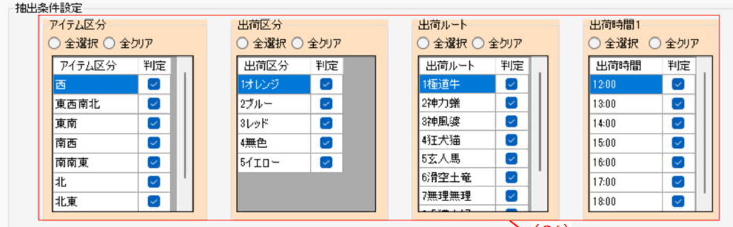
- Shipping time zone (1-hour segments): Visualizes the degree of order concentration before the cutoff time, utilized to determine the feasibility of advance work and to formulate an efficient truck docking arrangement schedule (berth reservation) based on the volume by time zone.
- Shipping route: Utilized to designate groups by direction (e.g., North Area, South Area) for company-owned fleets, or to predict the sorting workload at loading berths for each transport company, route delivery, and courier service, thereby preventing platform congestion.
- Shipping classification and item information: Used to grasp the conditions and required space for special tasks occurring during receiving and shipping, such as specifying packaging formats (like Oricon or cardboard) required for each destination, or distribution processing (tagging, pricing) and quality inspection.
3. Application Examples of the EIQ Matrix Aggregation Table in Operations
Item 6: Optimizing Picking Strategy via EIQ Matrix
When shipping destinations and products are matrixed in descending order of volume, the true test of skill is how to convert those figures into actual operational rules. For example, if a volume group of "0.5 pallets or more / PIC (volume generated in a single pick)" can be extracted from the data analysis results, this is defined as "pallet shipping."
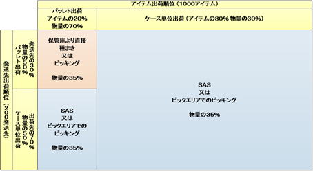
If this large-lot pallet shipping group is deliberately broken down into small units to be processed in the SAS (Sequence Assorting System) or in a standard picking area for small lots, traffic lines and labor will inversely increase, and efficiency will drop significantly. Therefore, it can be logically determined that it is optimal to batch-process 2 to 3 shipping destinations at once (sorting after total volume picking) using forklifts, etc., in a seeding area (sorting area) with wide aisles secured. On the other hand, the remaining small-lot groups can be segmented as suitable for storage and retrieval in the SAS or standard walking picking areas.
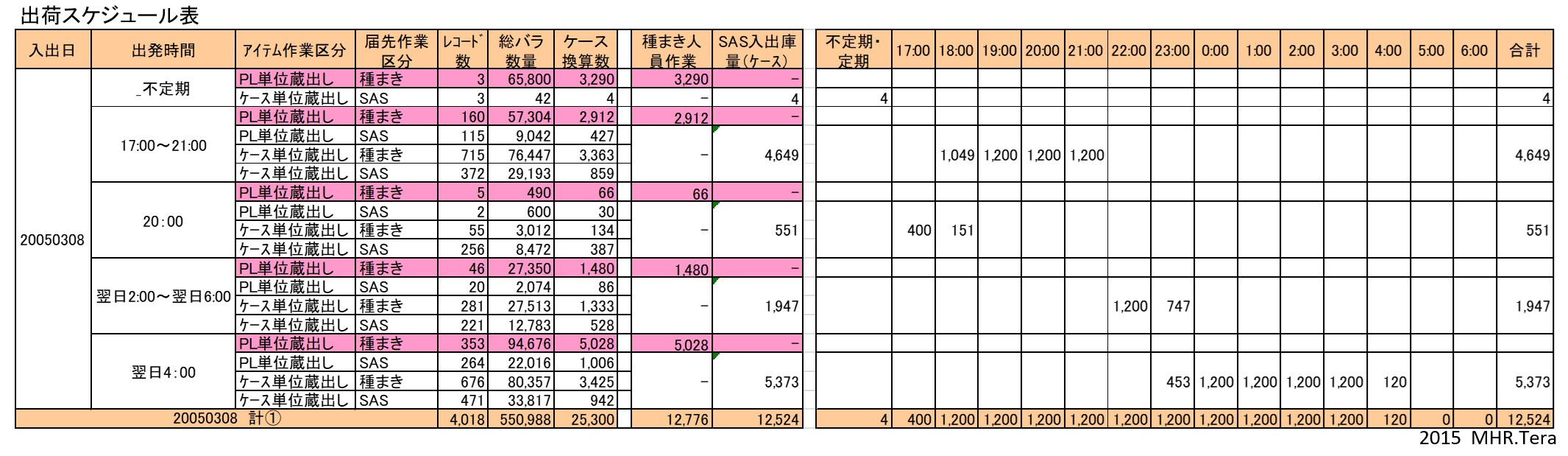
By using the EIQ matrix table in this way, it is possible to move beyond mere current situation analysis. It enables accurate calculation of the timing regarding which items should be replenished to which picking area (like SAS) and when, as well as the required number of containers for each area, allowing it to be incorporated into a practical daily work schedule. The accumulation of this process bears fruit in a waste-free facility scale calculation.