The "Shipping Data Aggregation" table above summarizes full shipping datasets by item field, appending conversion metrics omitted from raw shipping files: Case Conversions, Pallet Conversions, Cubic Volume Conversions, and Gross Weight Conversions.
Selecting the "Percentage Ratio %" radio button displays relative daily volume ratios setting the full shipping dataset as 100%.
Total destination and SKU counts in shipping data represent cumulative daily recurring shipment totals.
Shipping data contains 518 unique destinations and 4,594 unique SKUs (as listed in table summary).
The "Graph" displays data for date 2022/05/10:
Display 1 shows destination count, SKU count, and line item records.
Display 2 shows piece counts and case conversions.
Display 3 shows pallet conversions, cubic volume conversions, and gross weight conversions.
Full dataset analysis reveals diverse case pack variations spanning from 1 to 120 units per case.
Section 2 Traditional Calculation
ABC Analysis Applications in Tera Calculation (Traditional Calculation)
While standard ABC analysis sorts shipping data from high to low velocity and divides cumulative percentages into 3 tiers (A, B, C), Tera Calculation partitions datasets into 5 blocks (ranks) to provide flexibility in material handling equipment selection. Defined as "Traditional Calculation," this approach provides engineering justification for system design when compared against EIQ analysis outcomes.
1. Overall Dataset Aggregation & Parameter Additions
Appends practical logistics conversion metrics omitted from raw shipping data to establish a comprehensive macro picture of the distribution center.
- Appended Conversion Parameters: Case conversion, Pallet (PL) conversion, Cubic volume conversion, and Gross weight conversion.
- Estimating Case Dimensions: When raw shipping data lacks case dimensions, physical dimensions are estimated from case cubic volume assuming a standard aspect ratio of Length 5 : Width 4 : Height 3.
- Data Characteristics: Visualizes full dataset characteristics, revealing wide variations in case pack quantities ranging from 1 to 120 units.
2. Aggregation by Shipping Unit and Rank Classification
In logistics system design, segregating "Case Shipping" from "Piece Shipping" is critical because storage systems and handling procedures differ fundamentally between formats.
Categorization by Shipping Unit
- Case Shipping: Order line records dispatched as full case units.
- Piece Shipping: Order line records dispatched as loose piece units.
- Case-Piece Mixed Shipping: Single order line records calling for "1 full case + 3 loose pieces". Mathematically, these lines are split into 1 case record and 1 piece record, incorporated separately into respective rank calculations.
Equipment Allocation via 5-Rank Aggregation
Subdividing ABC analysis into 5 blocks creates operational flexibility when assigning material handling equipment.
- Example: Simplifies engineering evaluations such as "combining Ranks A1 and A2 into mobile racking" or "assigning Ranks A2 and B to static selective racking."
- System Consistency: Aggregation boundaries are engineered to align seamlessly with EIQ matrix table partition blocks.
3. Utilizing Pareto Charts (ABC Distribution)
Pareto distribution charts evaluating individual SKUs by sales value or physical volume can be displayed for reference.
- Observations: While monetary value-based analysis provides value for procurement and sales management, physical volume-based rank aggregation serves as a far stronger engineering justification when designing logistics equipment systems.
Subsection 1 Overall Dataset Aggregation
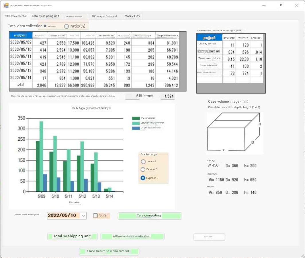
While raw shipping files contain case volume data, physical dimensional concepts are absent.
Case volume models project physical dimensions using a standard aspect ratio of Length 5 : Width 4 : Height 3.
Because cubic volumes are calculated, linking external master files containing actual case dimensions to shipping datasets reveals exact physical SKU sizes. Tera Calculation estimates case dimensions assuming external master files are unavailable.
Case shipping and piece shipping require different storage setups and picking workflows.
Because the overall data aggregation screen does not segregate case and piece shipping formats, equipment allocation cannot be performed directly; it serves as macro reference data for system design.
Subsection 2 Aggregation by Shipping Unit
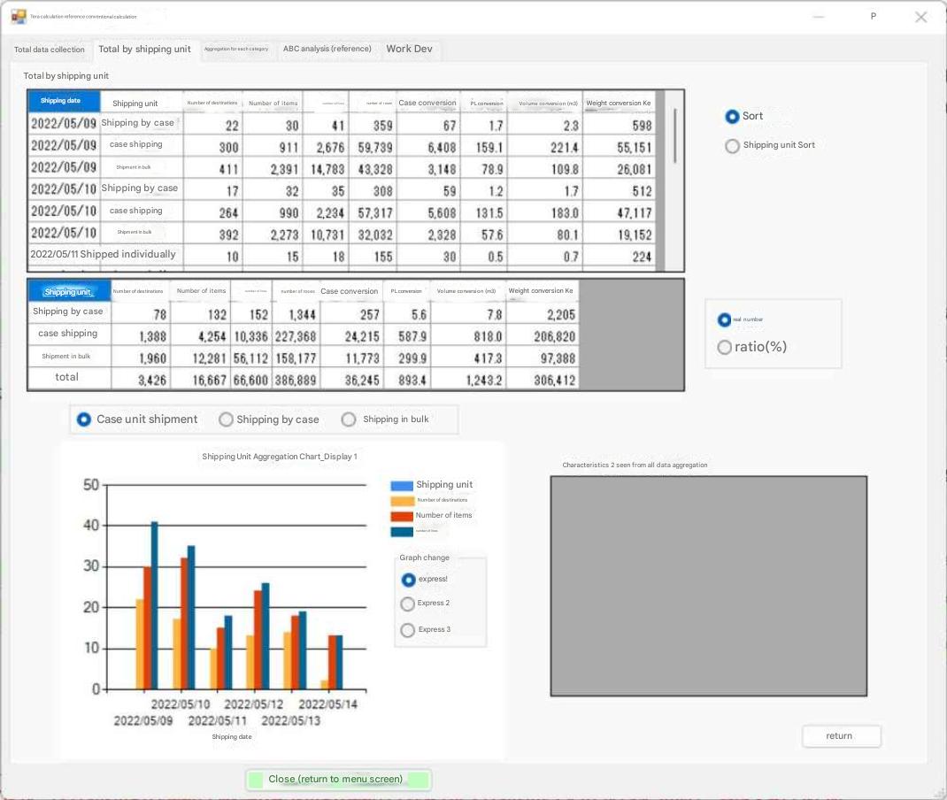
Table interpretation follows the same format as the Traditional Calculation screen.
Summarizes datasets segregated into Case Shipping and Piece Shipping.
Normally, order line records calling for case shipping dispatch full case units; piece shipping lines behave similarly.
Rarely, a single order line record requests 1 case plus 3 additional loose pieces; this represents a case-piece mixed shipment.
Case-piece mixed lines are processed as 2 separate dispatches (1 case record and 1 piece record), incorporated into case and piece rank calculations respectively.
Note:
Following rank aggregation, case-piece mixed values no longer appear as separate items.
While overall data aggregation notes state "case shipping and piece shipping differ in storage setups and workflows," they also differ fundamentally in physical volume throughput.
Aggregation by shipping unit alone remains insufficient for equipment allocation, serving as reference data during initial system engineering.
Subsection 3 Rank Aggregation
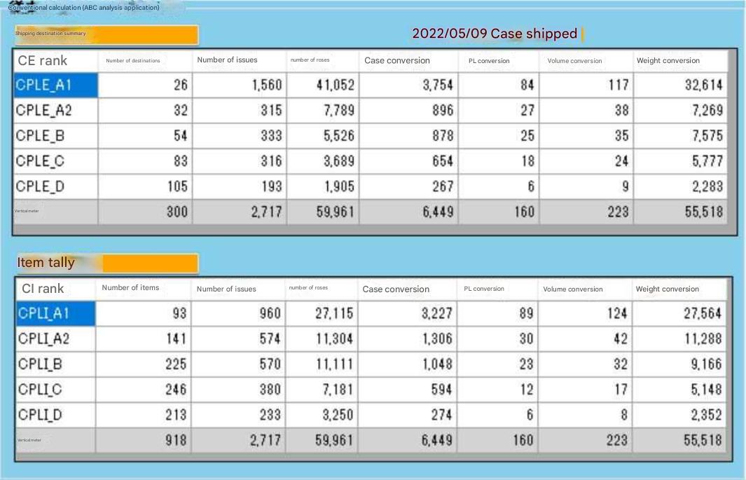
The table above corresponds to screens displayed in "Tera Calculation 1: Shipping Data Analysis".
Extracts and aggregates case shipping datasets; identical summaries can be generated for piece shipping.
Subdivides ABC analysis into 5 rank blocks rather than standard 3-tier partitioning.
Planners can verify shipping throughput per rank block using converted physical metrics (cases, pallets, cubic volumes) alongside piece quantities.
Because partition boundaries align with EIQ matrix tables, aggregation outputs match EIQ matrix results exactly.
Because the table above segregates shipping units and establishes 5-tier rank partitioning, material handling equipment can be assigned easily.
Storage equipment allocation uses full-period dataset averages (refer to Chapter 3 Tera Calculation 1: Shipping Data Analysis, Section 2 Equipment Allocation) alongside SKU summary data.
Partitioning datasets into 5 blocks creates operational flexibility—such as combining blocks CPLI_A1 and CPLI_A2 for mobile racking, or assigning blocks CPLI_A2 and CPLI_B to static selective racking.
Subsection 4 ABC Analysis (Pareto Chart)
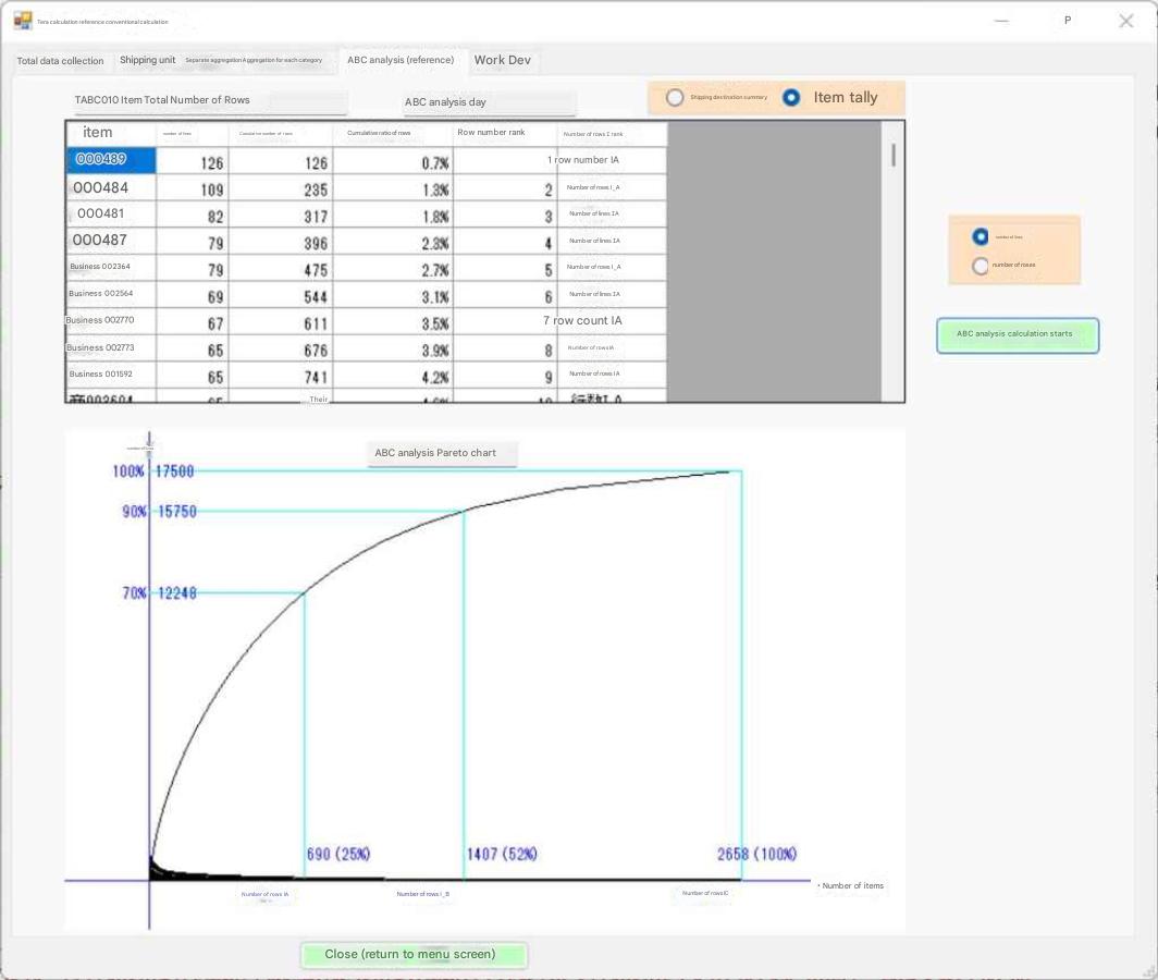
The table above displays standard ABC analysis for reference.
Presents sorted SKU rank order tables used to plot Pareto distribution charts.
Case shipping and piece shipping are aggregated separately.
Some analytical models express ABC distributions using SKU sales revenue values. While monetary analysis offers valuable insights for procurement and sales teams, it provides weak technical justification when determining material handling equipment specifications during logistics system design.