Section 1 EIQ Matrix Calculation (Analytical Aggregation)
This section explains "EIQ Matrix Calculation (Analytical Aggregation)", the core essence of shipping data analysis.
1. Difference Between Conventional Calculation and EIQ Matrix Calculation
There is a definitive difference between conventional logistics analysis (such as ABC analysis) and the EIQ matrix analysis proposed by Tera Calculation.
- Conventional Calculation (ABC Analysis):
- Because item aggregation and destination aggregation are performed independently, the interrelationship between the two remains unknown.
- It is impossible to grasp "which rank of products flows to which rank of shipping destinations."
- EIQ Matrix Calculation (Tera Calculation):
- Aggregates data by cross-linking "Item Rank (5 tiers) × Destination Rank (5 tiers) = 25 Blocks".
- This allows precise measurement of material volume flowing from a specific Item Rank (Equipment / Storage Type) to a specific Destination Rank (Shipping Area).
2. Insights Derived from the EIQ Matrix Table
Utilizing this matrix table significantly simplifies detailed specification planning for distribution centers.
- Grasping Workloads: Picking frequency, total piece count, volume, and weight can be verified across ranks.
- Equipment Optimization: Accurately calculates block-by-block item counts requiring flow racks, as well as replenishment case and pallet quantities.
- Unit Conversion Flexibility: All numerical values are converted from piece counts, allowing seamless toggling between units like cases, pallets, volume, and weight.
3. Reading Rank Notation Symbols
To prevent confusion, explicit rules are established to identify aggregation targets at a glance.
Example: "CケE_A1" (In Japanese notation: C-Cs-E_A1)
- 1st Character: "C" Case Shipping / "B" Piece Shipping
- 2nd Character: Criteria field used for ranking ("ケ" / "Cs" = Case Conversion)
- 3rd Character: "E" Destination Rank / "I" Item Rank
- 4th Character: "A1" Specific Rank Name
→ Meaning: Case Shipping Destination Rank A1.
4. Analytical Operation Steps
On the Tera Calculation 1 screen, analysis is processed through the following steps:
- Select Characteristic: Pick a target date by specifying a date or selecting characteristics like "Peak Case Shipping Day".
- Specify Category & Unit: Select Case/Piece, Actual Value/Ratio (%), and Display Unit (Piece, Volume, etc.).
- Condition Filtering: Filter target data using checkboxes for item categories, shipping routes, or shipping categories.
- Execute: Click the Start button to output results to the DataGridView (table).
Observations and Important Notes
- Visualization: Because massive datasets (over 400 destinations, over 4,000 items) cannot be deciphered using standard EIQ tables, grouping via matrix tables or EIQ Scatter Plots (for visual dispersion assessment) is exceptionally effective.
- Documenting Metadata: When clipping tables for reports or presentations, always include "Shipping Method", "Shipping Date", and "Display Unit" above the table to avoid future confusion.
Subsection 1 Difference Between Conventional Calculation and EIQ Matrix Calculation
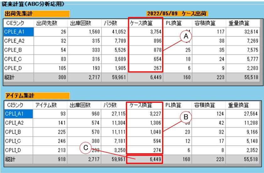
In Tera Calculation, calculations aggregated using ABC analysis methodology are referred to as conventional calculations.
While ABC analysis divides ranks into 3 categories for separate item and destination aggregations, Tera Calculation divides ranks into 5 categories for item and destination aggregations.
In conventional calculations, while the overall totals across items and destinations match, there is no structural link between item aggregation and destination aggregation. Consequently, conventional calculations cannot reveal how items of Item Rank A1 are allocated across destination ranks.
When calculating throughput volumes across processes or designing distribution center scale and operations, dataset linking destinations and items is essential.
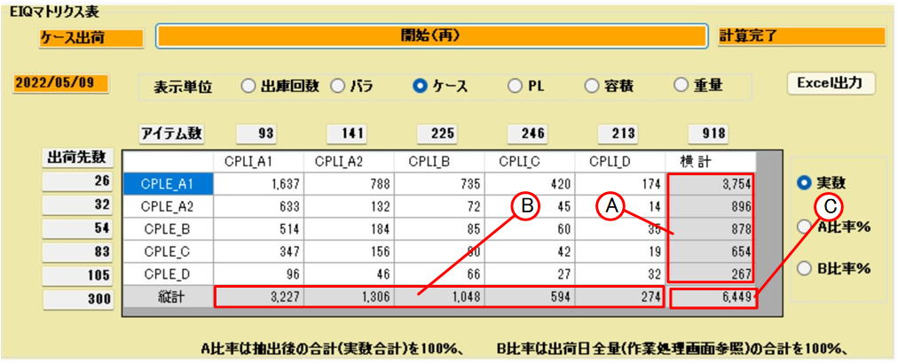
Tera Calculation proposes a method of linking item ranks and destination ranks, dividing and aggregating throughput across Item Rank 5 × Destination Rank 5 = 25 Blocks. Tera Calculation names this summary matrix the EIQ Matrix Table.
Furthermore, Tera Calculation can display Row Count (retrieval frequency), Piece Quantity, Case Conversion, Pallet Conversion, Volume Conversion, and Weight Conversion within the same rank matrix boundaries.
Through this EIQ Matrix Table, for example, one can easily read:
For Item Rank A1 items in the picking flow rack area, how many picking operations occur and what is the total piece count?
What is the corresponding cubic volume, and how many shipping containers are needed?
How many cases of replenishment are required from the storage area to the flow racks, and how many pallets are moved when transported as mixed pallets from bulk storage?
All these answers can be read seamlessly from the EIQ Matrix Table.
In the EIQ Matrix Table, display unit Piece means Piece Quantity, Case means Case Conversion, PL means Pallet Conversion, Volume means Volume Conversion, and Weight means Weight Conversion.
Please remember that henceforth, all material throughput units other than raw piece quantity represent converted units calculated from raw piece counts.
(When the term "Case" appears, it signifies Case Conversion).
As noted earlier, the EIQ Matrix Table is an aggregation matrix divided into 5 × 5 = 25 blocks; horizontal totals represent destination volume aggregations, while vertical totals represent item volume aggregations.
If the EIQ Matrix Table display unit is set to PL Conversion, horizontal totals match PL conversions in conventional item summaries, and vertical totals match PL conversions in conventional destination summaries. Matrix aggregation and conventional calculations are dynamically linked, displaying identical totals. The same holds true for destination counts and item counts.
Subsection 2 Relationship Between Conventional Calculation and EIQ Matrix Calculation
Because conventional calculations summarize destinations and items independently,
the relationship between destination throughput and item throughput remains unknown.
EIQ Matrix Aggregation,
reveals exact material volume for Item Rank A1 heading to Destination Rank A1, aggregating throughput with structural cross-linking between destinations and items.
Observations:
Through this EIQ Matrix Table,
one can precisely grasp how much volume flows from each Item Rank (Equipment / Rack Type) to each Destination Rank (Shipping Area).
The EIQ Matrix Table allows specifying extraction criteria to display dataset subsets matching target conditions.
Looking at summary tables often causes confusion regarding Case Shipping Item Rank A1, Case Shipping Destination Rank A1, Piece Shipping Item Rank A1, Piece Shipping Destination Rank A1, etc.
To eliminate this confusion, notation symbols are formatted so table contents can be identified at a glance.
Meaning of Rank Symbol "CケE_A1" (C-Cs-E_A1):
1st Character: "C" for Case Shipping, "B" for Piece Shipping.
2nd Character: Data field used for ranking:
"行" (Row) = Row Count (Retrieval Frequency), "バ" (Pce) = Piece Quantity, "ケ" (Cs) = Case Conversion, "PL" = Pallet Conversion, "容" (Vol) = Volume Conversion, "重" (Wt) = Weight Conversion.
3rd Character: "E" for Destination Rank, "I" for Item Rank.
4th Character: "A1" for A1 Rank, "A2" for A2 Rank, "B" for B Rank, "C" for C Rank, "D" for D Rank.
Therefore, rank symbol "CケEA1" indicates Case Shipping, ranked by Case Conversion, Destination Rank A1.
Observations:
When clipping EIQ Matrix Tables for insertion into separate report documents,
always note "Shipping Method (Case Shipping)", "Shipping Date (2022/05/09)", and "Display Unit (Case)" above the clipped table. Otherwise, it becomes impossible to determine what the summary represents.
Difference Between EIQ Table and EIQ Matrix Table
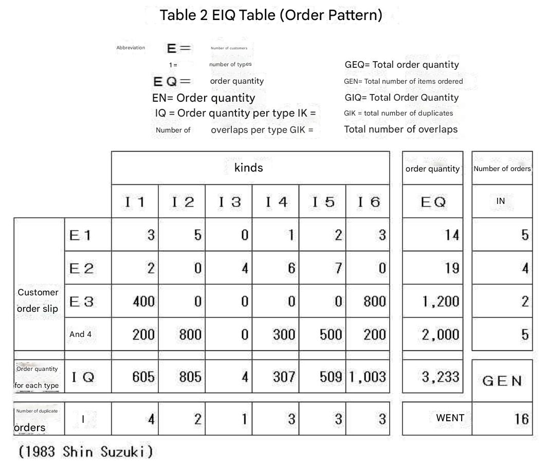
In principle, system engineering should be conducted by reviewing volume flow of which specific items go to which specific destinations; Mr. Susumu Suzuki introduced this format as the EIQ Table.
When destination counts are around 50 and item counts around 100, creating and analyzing a raw EIQ Table is indeed feasible.
However, for shipping datasets like this case—with over 400 destinations and over 4,000 items—an uncompressed EIQ Table exceeds the size of a large room and is completely decipherable.
In Tera Calculation, we devised an aggregation method that groups the EIQ Table by rank tiers, naming this the EIQ Matrix Table.
Additionally, there is a method of plotting the EIQ Table as points on a scatter chart. For 400 destinations and 4,000 items, plotting them visually on screen with horizontal scrolling allows observing EIQ dispersion patterns.
In Tera Calculation, we name this visualization the EIQ Scatter Plot (refer to Tera Calculation 4_Reference EIQ).
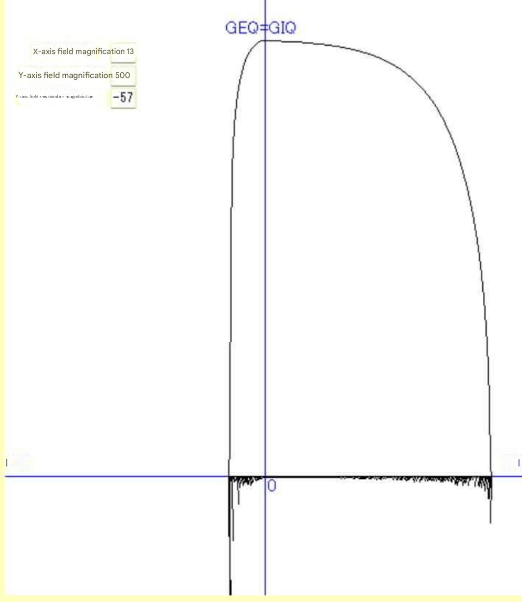
Next, we introduce the EIQ Graph created by Mr. Susumu Suzuki. This graph represents cumulative destination volume and cumulative item volume as curves, destination retrieval frequency and item retrieval frequency as bar charts, illustrating full-day volume profile in a single unified diagram (refer to Tera Calculation 4_Reference EIQ).
Please review EIQ Tables and EIQ Graphs in dedicated reference publications.
Subsection 5 Data Analysis & Aggregation
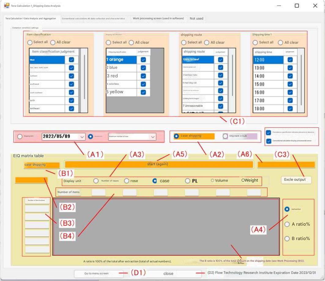
Initial screen of Tera Calculation 1.
At (A1), clicking the "Shipping Date" radio button aggregates by specified date; clicking "Characteristics" allows selecting peak characteristics like Max Row Count Day, Max Case Shipping Day, or Max Piece Shipping Day.
At (A2), radio buttons provide single selection between Case Shipping or Piece Shipping.
At (A3), radio buttons select 1 of 6 display units including Retrieval Frequency, Piece Quantity, etc.
At (A4), radio buttons select between Actual Value or Ratio (%). After making selections (A1) through (A4):
At (A5), click the Start button to execute processing.
At (A6), processing progress status is displayed in the text box.
Following calculation:
(B1) displays target Case Shipping / Piece Shipping category,
(B2) displays Shipping Date,
(B3) displays Destination Count,
(B4) displays Item Count, and
(B5) outputs the EIQ Matrix Table to the DataGridView (table).
The Matrix Table can display either Actual Values or Ratios (%).
Ratio A % displays each rank percentage setting filtered subset total (actual total) as 100%; Ratio B % displays each rank percentage setting total full-day volume as 100%.
At (C1), checkboxes select target conditions from 4 shipping data condition fields (multiple selections allowed). Data records unselected in checkboxes are excluded from EIQ Matrix Table calculations.
At (C3), Excel Output exports the EIQ Matrix Table to an Excel spreadsheet file.