Section 2 Shipping Data Processing

1. Data Import and Basic Conversion

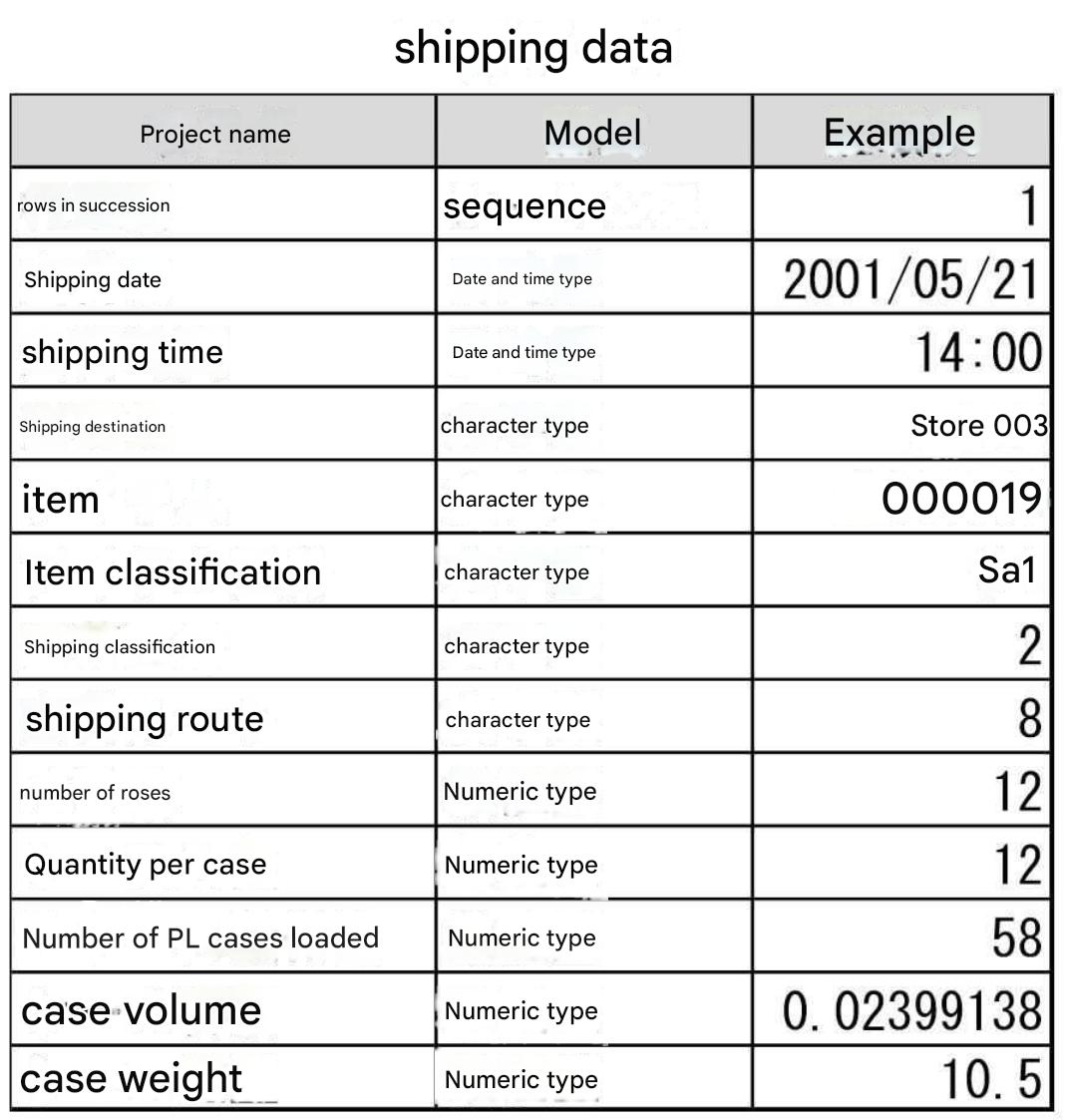
First, Excel-formatted shipping data is imported into Microsoft Access to create the "T000_Shipping Data" table.

Immediately following import, essential converted values required for logistics design are calculated for every record (row):

• Case Conversion: Piece Quantity ÷ Quantity per Case
• Pallet (PL) Conversion: Case Conversion ÷ Pallet Case Stacking Capacity
• Volume & Weight Conversion: Case Conversion × Case Volume (or Case Weight)

2. Separation of Case Shipping and Piece Shipping

Because storage locations and operational workflows differ between case-level units and piece-level units in a distribution center, these are strictly separated and aggregated independently.

• Case Shipping: Orders involving integer quantities of 1 full case or more. Products are retrieved from bulk storage racks and transported directly to sorting areas.
• Piece Shipping: Orders under 1 full case or involving fractional remainders. Products are picked from operational picking racks in the order fulfillment area.
  • Example: If an order requests 9 units of a product packed 5 per case, it is separated and counted as 1 case (Case Shipping) and 4 pieces (Piece Shipping).

3. 5-Tier Rank Assignment (Extension of EIQ Analysis)

A detailed 5-tier ranking system is executed—beyond conventional 3-tier ABC analysis—to optimize equipment allocation and operational workflows.

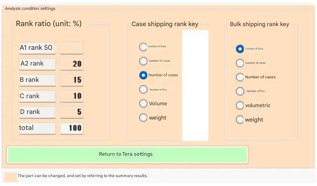
• Rank Ratios (Tera Settings): A1 (50%), A2 (20%), B (15%), C (10%), D (5%).
• Rank Criteria Keys:
  • Tera Calculation 1: Ranks Case Shipping based on "Case Conversion" and Piece Shipping based on "Row Count (Retrieval Frequency)".
  • Tera Calculation 2: Because storage capacity calculation is the primary goal, both are ranked based on "PL Conversion".

4. Creation of the "T200" Table

A consolidated master table named "T200" is generated by integrating all processed dataset fields (converted values, shipping categories, and rank attributes). Tera Calculation 1 and 2 perform analyses referencing solely this table, significantly increasing system processing speed.

5. Terminology Definitions and Operational Notes

• Definition of Retrieval Frequency: When both case and piece quantities are shipped within a single record, Tera Calculation counts this as "Retrieval Frequency: 2" to accurately reflect actual physical work burden.
• Bulk Storage In/Out: Warehousing stock into or retrieving stock out of primary storage rack space.
• Sorting vs. Picking: Allocating retrieved bulk goods to specific destinations is defined as "Sorting (Seed Picking)", while collecting individual items from picking racks is defined as "Picking (Item Picking)".
• Time-Window Considerations: Process peak periods are calculated backward based on dispatch deadline times. Upper-stream processes (such as picking) begin and finish earlier in the timeline.

Subsection 1 Shipping Data Import

Loading data into Access is called importing, while extracting data from Access is called exporting.
In "Tera Calculation 0", importing shipping data refers to taking Excel shipping data into Access to create the "T000_Shipping Data" table.
Because Access is initialized (emptied completely) prior to importing "T000_Shipping Data", only the "T000_Shipping Data" table exists in Access immediately after import.

Subsection 3 Categorizing Case Shipping vs. Piece Shipping

Distribution centers execute material handling operations in pallet units, case units, and piece units.
Tera Calculation separately analyzes and aggregates case-unit shipping versus piece-unit shipping because operational tasks and storage methods differ fundamentally between case and piece shipping.

Calculation Rules:
1. Quantities under 1 full case are Piece Shipping (Case Conversion < 1).
2. Quantities of 1 full case or more with no decimal fraction (e.g., 1, 5) are Case Shipping (Case Conversion >= 1 and Piece Quantity Modulo Quantity per Case = 0).
3. Quantities of 1 full case or more with decimal fractions (e.g., 1.1, 5.3) are Case/Piece Fractional Shipping (Case Conversion > 1 and Piece Quantity Modulo Quantity per Case <> 0).
4. In case 3, integer parts become Case Shipping and decimal fraction parts become Piece Shipping:
    Case Shipping Case Count = Int(Piece Quantity / Quantity per Case)
    Piece Shipping Piece Quantity = Piece Quantity - (Case Conversion * Quantity per Case)

Calculation Example:
When shipping 9 pieces of Product B (packed 5 per case) to Destination A, 1 case and 4 pieces are shipped.
Operational workflow in the distribution center proceed as follows:
The 1 full case is retrieved from bulk storage combined with identical items for other destinations and sorted in the sorting area.
The 4 loose pieces are picked from flow racks or medium-duty shelving in the picking work area.
Categorization between case shipping and piece shipping is calculated per individual record row.

Pallet-unit calculations can be derived from converted values whenever required.

Note:
While small-scale distribution centers may retrieve 2 cases and 3 pieces directly from storage simultaneously, Tera Calculation assumes a distribution center structure where case shipping and piece shipping operations are structurally separated.

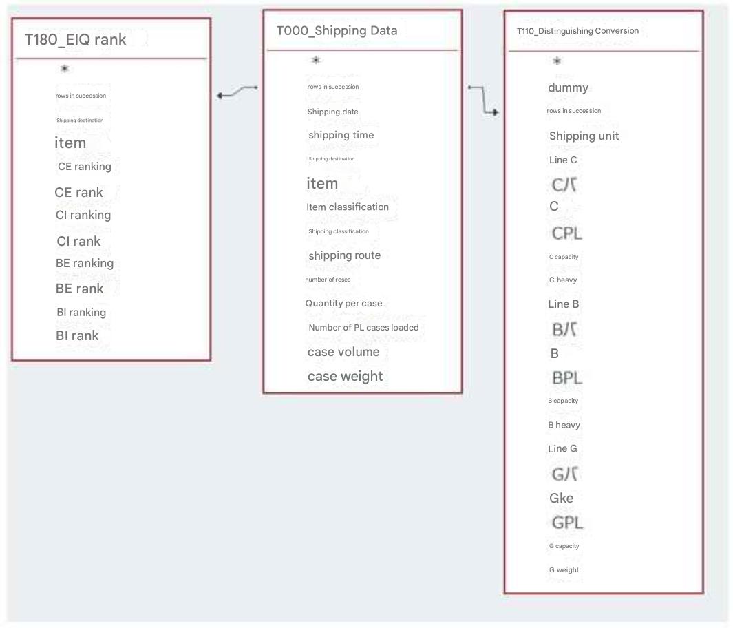
These calculation results are saved into the "T110_Category Conversion" table.

In the table above:
"C Row" denotes Case Shipping row count; "B Row" denotes Piece Shipping row count; "G Row" denotes combined Case + Piece Shipping row count.
The first character C, B, G represents shipping category; the second descriptor indicates Row = Row count, Pce = Piece count, Cs = Case conversion, PL = Pallet conversion, Vol = Volume conversion, Wt = Weight conversion.

Assigning Ranks to Shipping Destinations

Destination rank assignment utilizes the same 5-tier structure as item ranking.
Destination ranking applies the same percentage settings (Tera Settings) as item ranking.
Ratios and criteria keys used for destination ranking can be customized.

Creating the "T200" Table by Linking "T180" and "T110" to "Shipping Data"

After generating "T110_Category Conversion" and "T180_EIQ Rank",
these two tables are joined with "T000_Shipping Data" to create a new master table named "T200".
Utilizing the unified "T200" table simplifies SQL query construction and enhances processing speeds within the software.
Tera Calculation 1 and 2 perform analysis and aggregation referencing exclusively the "T200" table.
While omitting "T200" and joining "T110" and "T180" directly to "Shipping Data" during runtime offers the advantage of smaller Access database file sizes...

Subsection 5 Table File Layout

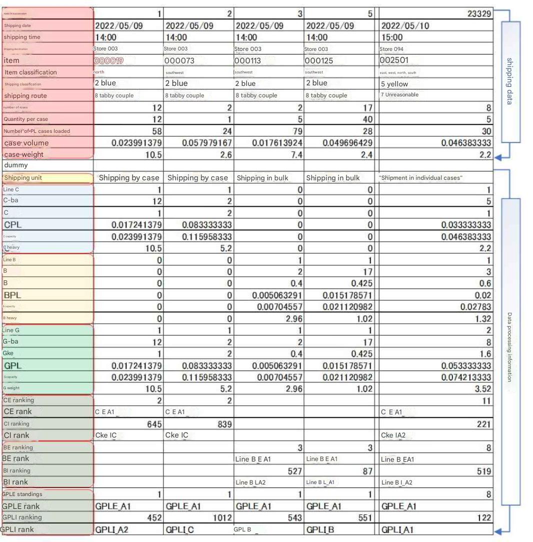
Fields from "Row Sequence No." through "Case Weight" contain identical content to raw shipping data.
"Dummy" is a Null field used during software calculation for inserting calculation tags.
(Null refers to a state containing no data value). Fields from "Shipping Unit" onward are generated by Tera Calculation 0.
"C Row" represents Case Shipping; "B Row" represents Piece Shipping; "G Row" represents combined Case + Piece Shipping.
Row 1 represents case shipping, where piece shipping fields contain 0 or Null; Row 3 represents piece shipping, where case shipping fields contain 0 or Null.
Fields from "CE Rank Order" to "CI Rank" contain rank data for case shipping; fields from "BE Rank Order" to "CI Rank" contain rank data for piece shipping used in Tera Calculation 1; fields from "GPLE Rank Order" to "GPLI Rank" contain rank data used in Tera Calculation 2 calculations.
While Tera Calculation 1 separates ranks between case and piece shipping, Tera Calculation 2 ranks combined case and piece throughput using pallets as the primary key (explained in Chapter Tera Calculation 2).
Row 23329 shows a "G Row" value of 2, indicating that Row 23329 required 2 retrieval operations (1 case retrieval + 1 piece retrieval).

Rank Assignment Keys

A rank assignment key is the numerical benchmark used for ranking (data aggregated by rank key prior to tier assignment).
If piece quantity is the key, data is aggregated and ranked by piece quantity.
If case count is the key, data is aggregated and ranked by case conversion.
Tera Calculation 1 targets peak shipping days, setting Row Count for piece shipping and Case Conversion for case shipping as default Tera Settings rank keys.
These are used to calculate shipping capacity from storage to order fulfillment areas.
Tera Calculation 2 targets overall shipping averages, using PL Conversion as the rank key for both piece and case shipping.
Distribution center scale calculations primarily involve storage volume computations from receiving to inventory (pallets, volume).
While selection of rank keys is widely debated, the author considers any valid logical choice acceptable.

Observations

In Tera Calculation 2_Distribution Center Scale Calculation, modifying ratios or rank keys allows immediate verification of changes in distribution center floor area (results display in 1–2 minutes).
Ranking case shipping and piece shipping separately is necessary because operational workflows differ between case and piece handling.
If case and piece shipping are not separated, aggregating by row count causes piece shipping to dominate top ranks, whereas aggregating by case conversion causes case shipping to dominate top ranks, creating a logical contradiction.
Tera Calculation selects a methodology that ranks case and piece shipping separately according to their respective operational characteristics.
However, during inventory calculations, averaging total shipping data (piece + case) is deemed most rational.
ABC analysis divides volume from high to low velocity into 3 tiers: A Rank 70%, B Rank 20%, C Rank 10%, but 3 categories feel insufficient.
In practical experience, 5 rank tiers allow appropriate equipment allocation and operational segmentation.

Specific Procedure for Rank Assignment

Example: Item Ranking for Case Shipping
1. Specify Item Rank Key.
Rank keys are volume comparison criteria: Shipping Frequency, Piece Quantity, Case Conversion, PL Conversion, Volume Conversion, Weight Conversion (weight is rarely used).
Tera Settings select Case Conversion for case shipping and Shipping Frequency for piece shipping.
2. Assign volume ratios to each rank.
Tera Settings establish 5 tiers: A1 Rank 50%, A2 Rank 20%, B Rank 15%, C Rank 10%, D Rank 5%.
3. Aggregate all records per item for case shipping.
Sort item totals in descending order of volume, assigning sequential rank numbers.
Calculate cumulative volume and cumulative volume ratios in order, assigning ranks per specified ratio thresholds.
Link these item ranks and sequence numbers to each record in the shipping dataset.
By linking, each shipping record displays its corresponding item rank and sequence order.
4. Calculate destination ranks for case shipping using the same method as step 3.
5. Calculate item ranks and destination ranks for piece shipping using the same method as step 3.
6. Reference "T180_EIQ Rank" table for rank classifications.

T180_EIQ Rank is an Access table name; CE Order denotes Destination Rank Order for case shipping; CI Rank denotes Item Rank for case shipping.

Subsection 6 Supplementary Notes on Shipping Data

Generally, Record Count = Retrieval Frequency in standard calculations, but Tera Calculation treats Record Count and Retrieval Frequency as distinct units.
Record refers to a line row in shipping data, whereas Retrieval Frequency refers to physical retrieval operations.
If 1 case and 3 pieces are shipped in 1 record, retrieval occurs once for case shipping and once for piece shipping.
Tera Calculation counts 1 record row as 2 retrieval operations.
Normally, storing goods onto racks is called putaway/inbound, and removing goods is called retrieval/outbound.
Using "inbound/outbound" for both storage space racks and work area picking racks causes confusion.
To avoid ambiguity hereafter, storing goods into storage racks is defined as "Bulk Putaway", and removing goods from storage racks is defined as "Bulk Retrieval".
Distributing retrieved bulk goods per destination is called "Sorting" (also termed Seed Picking). Storing retrieved goods onto work area racks (replenishment) and picking goods per destination from those racks is called "Picking" (Item Picking).
The term "Sorting" is frequently used loosely to include both Seed Sorting and Item Picking. In this document, Sorting = Seed Sorting, Picking = Item Picking, and Overall Sorting = Seed Sorting + Item Picking.
Tera Calculation handles distribution center facility systems and does not address vehicle transport/delivery after loading onto trucks. For transportation, please refer to separate publications.
Calculations in shipping data analysis use double-precision floating points (highest PC precision). However, because calculation results pass through multiple processing stages, minor rounding discrepancies are inevitable. (No erroneous displays have been identified at present).
Screen displays round numbers to integers for readability while software maintains double-precision internally.
Distribution centers require capacity to handle peak-hour workloads; when capacity is insufficient, operational countermeasures (such as advancing schedules or adding staff) are required. Summary totals during peak hours in Tera Calculation should be evaluated considering these peak operational countermeasures.

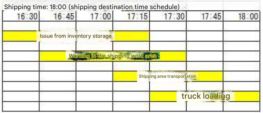
Peak time windows for each process stage are determined based on shipping dispatch times; shipping must be completed by designated deadline times. Therefore, note that start and end times for upstream processes shift earlier in the schedule.

Dedicated Fleet Delivery vs. Commercial Parcel Express
Dedicated Fleet Delivery is a distribution mechanism where shippers or carriers secure dedicated delivery routes and dedicated trucks for specific accounts.
Commercial Parcel Express is a distribution mechanism where logistics carriers maintain fixed delivery networks and trucks, and shippers request individual case delivery.